The FILTER() function enables you to filter data with the number of filters up to the max. number of columns
in a worksheet, sort the results using up to six keys and pre- or post-filter the data to find compound duplicates
consisting of up to 100 keys/columns.
Filter types include: Regex (regular expressions), patterns (with *, ?,~), "similar to" (fuzzy searches), all of the numeric
and literal =, <, >, relations, ranges, content length comparisons, empty cells, duplicates.
The function uses the following parameters:
=Filter(search-range, filters, hyperlink-path, options[, empty-string])
search-range
The "search-range" argument represents a range (or an array) with rows to filter. It can be of any size
up to the maximum number of columns in a worksheet minus one (as the 1st output column may additionally contain hyperlinks).
If there are any rows found in the search range, FILTER() returns an array with the corresponding number of columns.
If you specify the "hyperlink" option as described below and apply the Format > Hyperlink style
to the first column of the range when the returned array is, this first column will contain hyperlinks
to the original rows in "search-range".
Thus the filtered rows/records can be easily edited. After clicking a given link (or pressing SPACE) and completing editing
of the source data, you just click the "back" bookmark toolbar button (or press Alt+F11) to go back to browsing results in the same place.
filters
The "filters" argument represents a range or an array with filtering expressions for the subsequent
columns in the "search-range" range. Thus the number of cells in "filters" must not
exceed the number of columns in the "search-range" range. The n-th cell position
in this range/array is a filter expression for the the n-th column in the "search-range" data range.
If there is no filter for a given column, the corresponding filter cell can be left empty.
Entering filters in worksheet cells is easy: you can use the Format > Search Filter format style
for the desirable cells. This will display formatted filters with e.g. syntax coloring for Regex expressions and graphic sort
order indications.
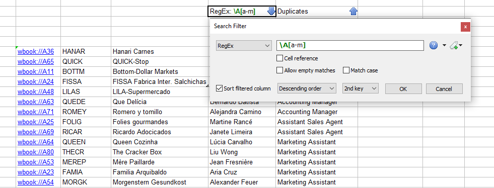
When editing such cells, GS-Calc displays a cell-aligned dialog box with all the filter specification and sort options:
 Example
The filter options are as follow:
- Cell reference - the filter text is cell reference (for the "between" filter type: two references)
- Allow empty matches - required by RegEx if you want to use expressions like \A\z
- Match case
- Word sort order - when sorting and searching for duplicates ignore punctuations and non-word characters
- Sorting and the sort key index - for a single column sorting it's always "1st key"; if you want to use multi-column sorting
you must specify subsequent key indices ("2nd", "3rd", ..."6th") for the other sorted columns. If there are repeated indices, FILTER()
returns the "#VALUE!" error code.
Note: The "duplicates" filters are handled slighly differently than the other filters. The "options"
parameter enables you to specify whether searching for duplicates should be performed before or after all other filters are applied.
You can also specify filters directly as text cells, e.g. if you want to generate them by your formulas.
hyperlink-path
The "hyperlink-path" argument represents a worksheet/workbook path that will be be used along with
cell references if the "include hyperlinks" options is specified (see below).
For example: sheet1, folder1\sheet1, c:\documents\[sample.gsc]sheet1
On the above example screen, the hyperlink path is left empty as both the data (A1:H100000) and the result
(=FILTER(A1:H100000, ...) are in the same worksheet.
options
The "option" argument is a number and can be 0 or a combination (a sum from 1 to 7) of the following:
- 1 - include hyperlinks to the original search-range data rows in the first column in of the FILTER() function results
- 2 - perform searching for duplicates AFTER all other filters are applied; by default the searches for duplicates are performed first
- 4 - as FILTER() is supposed to offer the best possible speed when handling very large tables, by default it doesn't create
calculation chains with formulas placed in the "search-range" range; if e.g. some column in the "search-range"
consists of formulas and you want to make sure FILTER() is executed after they're updated, add this "4" value
to options. Please note that this will result in significantly slower filtering.
The default value is 0.
Note: If you're using FILTER() for very large data sets and if you expect you'll be changing this (and
other) options frequently, use a cell reference for "options" in FILTER() instead of a hard-code value because re-editing the FILTER()
formula cell may activate the "Undo" for most of the target range and cause unnecessary delays before actual filtering.
empty-string
The optional "empty-string" argument represents a number or a string that the FILTER()
function is to return if no matching rows are found for the specified filters. If it's omitted,
FILTER() returns the "#N/A!" error code in such a case.
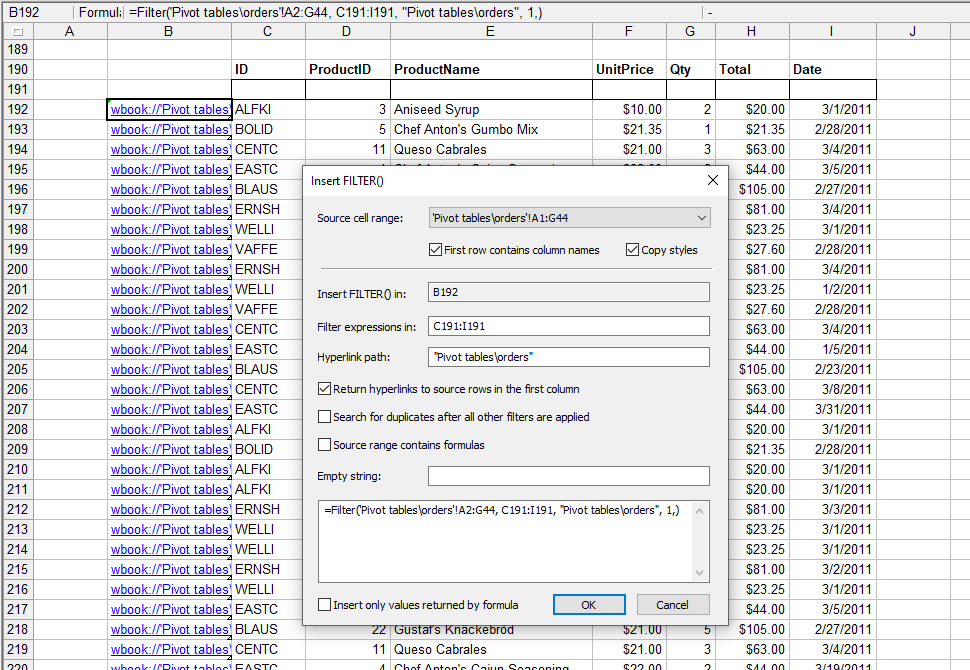
You can insert the Filter() function with just two clicks using the Insert > Filter() command.
The displayed "Insert FILTER()" dialog box determines the optimum parameters including the filters range and creates the formula. On the screen below the "Insert" command was used to filter data in the "sample.gsc -> orders " worksheet with a single "OK" click. It automatically copies the source styles, adds the necessary "hyperlink" and "filter expression" formatting.
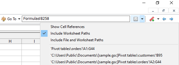
The source range 16 element list is a global list created and stored in the settings file. Subsequent source ranges are added
in a circular manner by clicking one of the following:
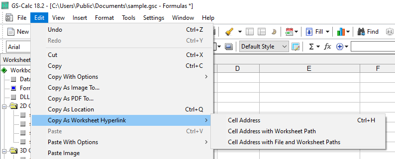
The "Copy as Location" menu command
The "Enter" toolbar button